Background
Cruising through Kaggle last week, I found a CSV of NFL play-by-play statistics. I get particularly excited about sports data so I started digging into this one right away. The data I found was compiled by Maksim Horowitz, Ron Yurko, and Sam Ventura. I originally found the CSV posted on Maksim's Kaggle page.
After reading a bit more I learned that they've created a really cool NFL API scraping tool called nflscrapR (written in R) that not only scrapes, cleans, parses, and outputs the CSV, but they also built expected point and win probability models for the NFL and have included this information in the CSV. Thanks to them for the work and sharing the data!
Motivation
There are a million different things one could do with this data, and indeed the people of Kaggle have done many things - from data cleaning to play call prediction. My particular interest, and what I'm going to focus on in this write up, is what type of offensive play (pass, run, punt, or field goal) teams are running by down and by location on the field.
In other words, we'll be able to answer questions like - What's the most common type of play called on the opponent's 20 yard line on any down? - What's the most common type of play called on the opponent's 20 yard line on first down? - Where on the field do most running plays starts when it's a third down?
The data...and some cleaning
The data is contained wholly within one large CSV. Sounds like a Pandas no-brainer to me. So let's first import Pandas and some other modules.
import pandas as pd
from bokeh.plotting import figure, show
from bokeh.models import ColumnDataSource, FactorRange, FixedTicker
from bokeh.io import output_notebook
from collections import Counter
from bokeh.transform import factor_cmap
from bokeh.palettes import Paired, Spectral
import itertools
pd.set_option('display.max_columns', 150)
output_notebook()
As you can seen I'm going to be using Bokeh for plotting, Counter from the collections module, and itertools as well. As is also obvious, I originally did this in a Jupyter Notebook that I've made available in my repository here.
Since they did a really nice job formatting the CSV, I can simply read the data into a dataframe without any other arguments.
filename = 'NFL Play by Play 2009-2017 (v4).csv'
df = pd.read_csv(filename)
A simple df.shape shows me that there are 407688 rows and 102 columns of data. Definitely something Pandas and Bokeh can handle. I trust that the data has been pretty well cleaned but I'm going to do my due diligence before I start calculating statistics on the data anyway.
I'm mostly interested in aggregating data by down so let's check how much null data exists in the 'down' column. Running
df['down'].isnull().sum()
shows me that 61154 rows of the 'down' column contain non-numeric data. Presumably, these instances are kickoffs and extra points or something where there technically isn't a 'down'.
NOTE: I'm making the assumption that the 'clean' data I'm investigating has properly inserted NaN values in rows where the 'down' data is bad. If I couldn't make this guarantee I'd probably do something like
pd.to_numeric(df['down'], errors='coerce').isnull().sum()to first try and convert everything in the column to a numerical value, inserting NaN where it can't, then count nulls and sum.
So let's drop all those columns.
# filter by team if desired
team = 'all'
if team == 'all':
    team_df = df
else:
    team_df = df.loc[df['posteam'] == team]

# drop rows will null in the 'down' column
team_df = team_df.loc[df['down'].notnull()]
NOTE: I've also included the ability to filter the data down by team (column 'posteam') in case looking at the data by team is of any interest. For this post I'm going to use data from all teams.
Now that I have the data I'm interested in, I'm going to count how many plays of each type there were as a final sanity check.
all_play_types = Counter(team_df['PlayType'])
NOTE: For those who don't know, according to the Python docs, '
Counteris adictsubclass for counting hashable objects'. In this case I'm passing it a Pandas Series (the 'PlayType' column) and it's counting all the different instances it finds in the column and returns aCountertype. It has adictinterface with each unique item found as the keys and the number of instances found as the values. For more info, see the Python docs.
For easier reading I'll put the results in table form:
| Play Type | No. of Plays |
|---|---|
| Pass | 158928 |
| Run | 120624 |
| Punt | 22003 |
| Sack | 10643 |
| Field Goal | 8927 |
| No Play | 21225 |
| QB Kneel | 3529 |
| Spike | 640 |
| Timeout | 12 |
| Kickoff | 2 |
| Half End | 1 |
For the most part, nothing really surprising except that there are 2 instances of 'Kickoff' on plays that actually had a down assigned. This is unexpected. Unless there's some obscure rule in football I'm unaware of it'd probably require some further investigation but since this is just for fun, I'm going to ignore it.
On with the analysis
Looking at play type by down
The first thing I want to do is a just a create a simple bar graph to see the breakdown of play type by down. I want to do this with a Bokeh vbar plot with nested categories. Here is great resource for working with categorical data in Bokeh - specifically nested categories.
If you're not familiar with Bokeh, most plots are driven by the ColumnDataSource which is a fundamental data structure of Bokeh. I'll leave the fine details of the ColumnDataSource for the reader to find here in the Bokeh docs, and suffice it to say in this post that the code below is just getting the data ready for loading into the ColumnDataSource object.
# list of downs I care about
downs = ['1','2','3','4']

# list of plays I care about
plays = ['Pass', 'Run', 'Punt', 'Field Goal']

# define x-axis categories to be used in the vbar plot
x = list(itertools.product(downs, plays))
# x = [('1', 'Pass'), ('1', 'Run'), ('1', 'Punt'), ..., ('4', 'Punt'), ('4', 'Field Goal')]

# create a list of Counters for each down--will include ALL PlayTypes for each down
plays_on_down = [Counter(team_df.loc[team_df['down'] == int(down)]['PlayType']) for down in downs]

# create a list of counts for each play in plays for each down in downs
counts = [plays_on_down[int(down)-1][play] for down, play in x]

# load the into the ColumnDataSource
source = ColumnDataSource(data=dict(x=x, counts=counts))
A little code goes a long way here. All I'm doing though is figuring out how many of each plays happened
on each down and then packing that into a ColumnDataSource. Now I'm ready to start configuring my vbar plot.
# get the figure ready
p = figure(x_range=FactorRange(*x), plot_height=350, plot_width=750, title='Play by Down',
           toolbar_location=None, tools='')

# create the vbar
p.vbar(x='x', top='counts', width=0.9, source=source, line_color='white',
           fill_color=factor_cmap('x', palette=Spectral[4], factors=plays, start=1, end=2))
p.y_range.start = 0
p.x_range.range_padding = 0.1
p.xaxis.major_label_orientation = 1
p.xaxis.axis_label = 'Down'
p.yaxis.axis_label = 'Number of Plays'
p.xgrid.grid_line_color = None
show(p)
All the hard work here is done by the FactorRange method, which is a nice touch from the Bokeh folks. It automatically figures out the offset and width each bar needs in each category taking into account the number of levels and padding. It's far less work than manually doing it with matplotlib. The factor_cmap distributes my colors to each nested vbar in each level - another very handy method for working with nested vbar plots. Here's the result:
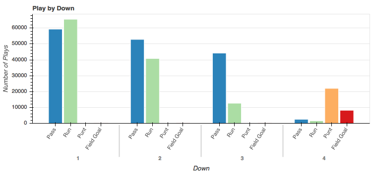
So nothing too surprising here but there are a few things worth nothing.
- Teams elect to run on first down by a slight majority.
- Not many teams elect to punt or attempt a field goal on downs 1-3. That's good, I guess.
- Passing becomes more and more popular as you use up your downs.
- On third down, pass attempts outnumber run attempts at almost a 4 to 1 clip. This is likely out of increased desperation to make a first down.
That last point makes me wonder at what point teams elect to run on third down. What's the break point in yards to go where passes become more popular than runs? Let's find out!
Looking at play type on third down as a function of yards to go for a first down
Let's first collect the data I need.
# define range of yards to go I want to look at
y2g = range(1,25)

# filter down the total team_df to just third downs
team_df_d3 = team_df.loc[team_df['down'] == 3]

# create list of Counters of PlayType for each yard in my rage of interest
plays_on_d3 = [Counter(team_df_d3.loc[team_df_d3['ydstogo'] == yrd]['PlayType']) for yrd in y2g]

# x-axis is y2g, defined above
x = y2g

# extract the run count for each yard
y_runs = [play['Run'] for play in plays_on_d3]

# extract the pass count for each yard
y_pass = [play['Pass'] for play in plays_on_d3]

# get the figure ready and put my lines on it
p = figure(title='Third Down Play Type by Yard to Go', toolbar_location=None, tools='',
           plot_height=350, plot_width=750)
p.line(x, y_pass, color='#2b83ba', legend='Pass', line_width=4)
p.line(x, y_runs, color='#abdda4', legend='Run', line_width=4)
p.legend.location = 'top_left'
show(p)
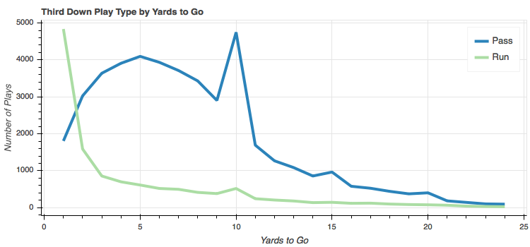
Let's first explain away the spikes. The huge spike at 10 yards is most likely from two previous unsuccessful attempts to move the ball forward, which is quite common. I believe the story is similar for the spikes at 15 and 20 yards with a penalty or two moving them back.
This rest of this chart might be easier to interpret by taking looking at the ratio of passes/run by yards to go.
# simple ratio of pass count/run count for each yard
y = [play['Pass']/play['Run'] for play in plays_on_d3]
p = figure(title='Third Down Pass/Run Ratio by Yards to Go', toolbar_location=None, tools='',
           plot_height=350, plot_width=750)
p.line(x, y, color='#2b83ba', line_width=4)
p.xaxis.axis_label = 'Yards to Go'
p.yaxis.axis_label = 'Pass/Run Ratio'
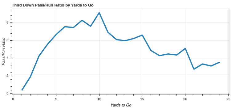
So it looks like the breakpoint is just under two yards to go. With one yard to go, runs outnumber passes nearly 3 to 1. Beyond two yards, passes are significantly more popular than runs. To be honest this surprised me a bit. I definitely expected more passes on third down, but this ratio jumps up fast! Even at just three yards to go, we see passes outnumbering runs at over 4 to 1 and nearly 8 to 1 at as little as 6 yards to go. Guess teams are desperate for that first down!
I'm not going to do it here but it'd be interesting to see what the average yardage gain is on third down runs.
Looking at plays by position on the field
Now I want to look at what kind of play is being run as a function of offensive position on the field. So first I'll collect the data I need.
# define range of yard lines I'm interested in.
yrdline = range(0,101)

# create list of Counters for every yard line on the field.
plays_on_yrd = [Counter(team_df.loc[team_df['yrdline100'] == yrd]['PlayType']) for yrd in yrdline]
This is similar to what I did earlier. I'm just collecting a list of Counters for each 'PlayType' at each yard line on the field. Let's plot it.
# extract counts of each PlayType I'm interested in for each yard
y_pass = [play['Pass'] for play in plays_on_yrd]
y_runs = [play['Run'] for play in plays_on_yrd]
y_punt = [play['Punt'] for play in plays_on_yrd]
y_fg = [play['Field Goal'] for play in plays_on_yrd]
p = figure(title='Plays by Yard Line', toolbar_location=None, tools='',
           plot_height=350, plot_width=750, x_range=(1,99))
p.line(x, y_pass, color='#2b83ba', legend='Pass', line_width=4)
p.line(x, y_runs, color='#abdda4', legend='Run', line_width=4)
p.line(x, y_punt, color='#fdae61', legend='Punt', line_width=4)
p.line(x, y_fg, color='#d7191c', legend='Field Goal', line_width=4)
p.legend.location = 'top_right'
p.xaxis.axis_label = 'Yard Line (100 is team\'s own goal line)'
p.yaxis.axis_label = 'Number of Plays'
p.xaxis.ticker = FixedTicker(ticks=list(range(0, 101, 5)))
show(p)
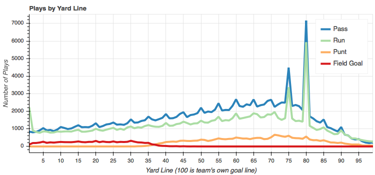
You can think of this plot as a football field where the offense is always going from right to left. So the 100 yard line is the offense's own goal line and the 0 yard line is the end zone the offense is trying to reach.
Again we see some spikes at the offense's own 20 and 25 yard lines (80 and 75, respectively, on the chart). This is because most plays start at these locations after a touch back from a kick off. The small spikes at 5 yard increments is interesting and I don't really have a good explanation other than to think that whoever recorded the yardage data liked rounding to the nearest 5 if it was close. Anyone else have any other ideas?
We're looking at total plays here, so it's easy to see that passes are favored over runs for pretty much the entire length of the field. The exceptions being very close to either end zone. Not surprising since when you're close to your own end zone, you don't want have the QB drop back and risk a safety. And not surprising at the other end of the field either. A little brute force with a draw play or QB sneak within a yard or two of the end zone is quite common.
Normalized by number of plays at each yard line
I'd like to look at this same data but normalize it by the total number of plays at each yard line. In other words, I want to see what fraction of plays were passes, runs, punts, and field goals at each yard line.
I pretty much have all the code I need to get there. I just need to add a function to sum up the total number of plays that I'm counting at each yard line. I'm not going to put the code here since it's very similar to the above but you can find it in the notebook.
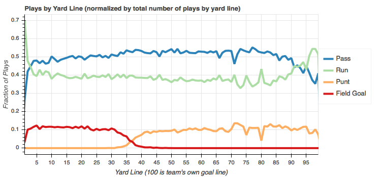
Ok, so same data but a little easier to read. In this plot the break point between punts and fields becomes obvious - somewhere around the 36-37 yard line. It's also interesting to note that it appears that as field goals begin to take a fraction of the overall play count, it's the passing plays that makes the room for it and runs stay pretty much steady. I would venture to guess that it's conservatism by the offensive play caller that causes this. They know they're in field goal range and can all but guarantee 3 points if they can keep possession. No sense in risking the interception.
I'm curious how this varies by down so let's find out!
First down
For the interested readers, you can find the code in the notebook. It's exactly the same code, but I'm filtering to dataframe to just plays on down one. Here's the resulting plot.
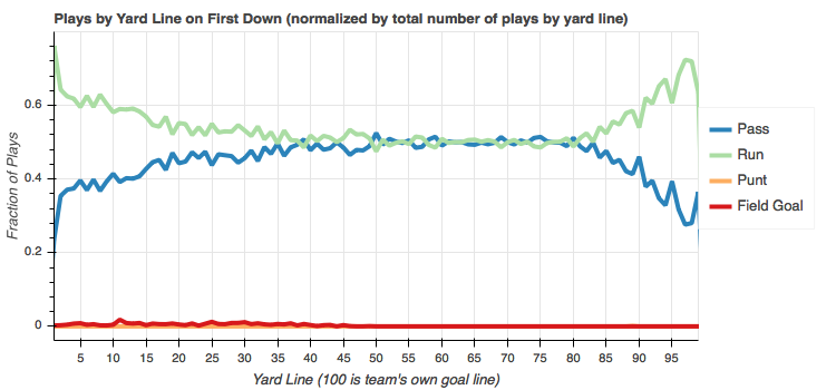
Between the offense's own 20 yard line and the defense's 35 yard line it's pretty evenly split between passes and runs. When backed up against their own end zone, the offense overwhelmingly elects to run. Within the defense's 35 yard line, run plays become more and more common. Again, conservative play calling to keep possession is likely the cause here. You can see a trickling of field goals on first down, most likely at the end of the half of the end of the game.
Second down
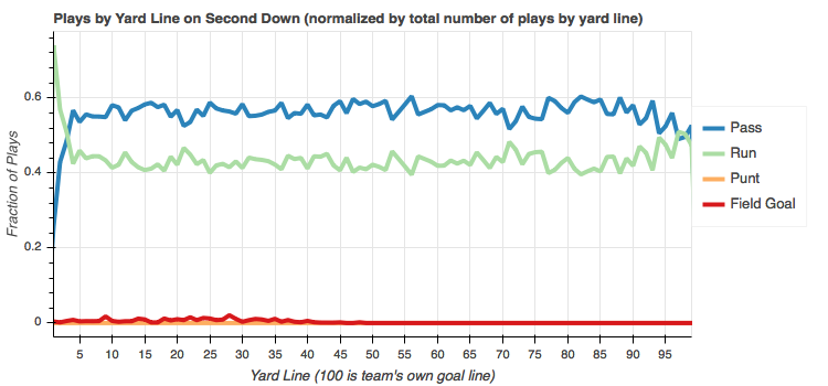
Interesting. Passes are consistently chosen more often on second down regardless of field position. The exception being within a few yards of the end zone. Makes sense.
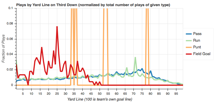
Third down
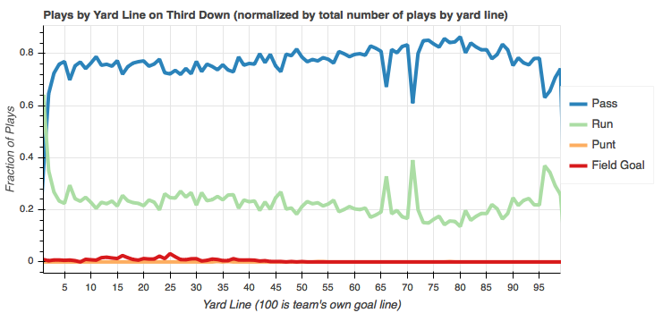
Wow! Passes are overwhelmingly favored on third down from anywhere on the field except the 1 yard line. I'd guess the spikes at the offense's own 29 yard line and 34 yard line are run efforts made with one yard to go on the first possession after a touch back.
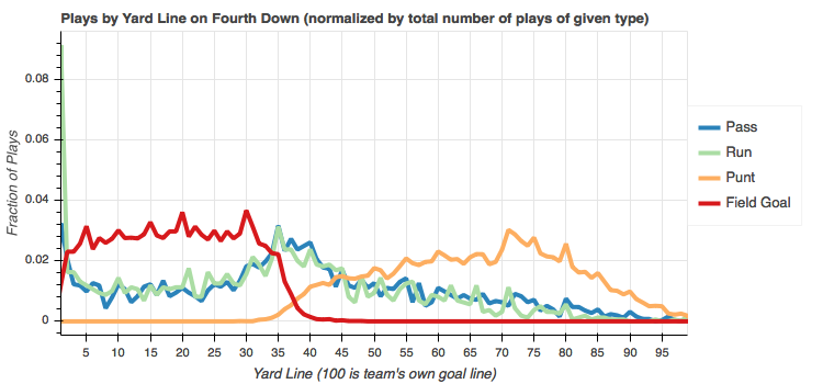
Fourth down
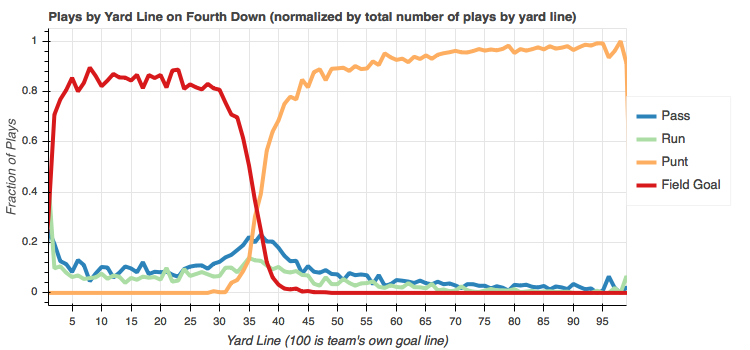
No surprise that punts are almost guaranteed on fourth down beyond the 45 yard line and field goals are overwhelmingly chosen within the 30 yard line. Between the 30 and 45 appears to be an area of indecision. I'm sure it depends a lot on the game situation but, comparatively, there's a fairly even split between all four play types in that range. Another point to note is that on the 1 yard line, even on fourth down, teams really want that touchdown.
Normalized by the total count of a given type of play
Now instead of normalizing by the total number of plays at a given yard line, I'm going to normalize each play type at each yard line by that play type across the entire field. In other words, the fraction on the y axis will be relative to each play type across the entire field. So the sum of values that make up each line will sum to 1. Doing this will allow me to see, for example, of all pass plays across the the entire length of the field, what fraction of them occurred at a given yard line.
Let's take a look. Again, the code will be in the notebook. The only difference here is that I need a function to sum up the total number of plays of a given play type across the entire field.
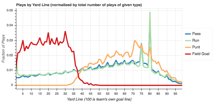 So remember, the fractions represent fractions of a given type. So looking at the runs, for example, I can see that nearly 5% of all run plays start at the 20 yard line. Same story for the passes and again this is because of how often plays start here from touch backs. It it worthy to note that since the majority of plays start here, you can see a lot of action between the 20 and 30 yard lines and it decreases and you move up the field. This is expected since continuing that far down the field requires several first down conversions.
It's interesting to note that most punts occur at the 29 yard line. Likely because of unsuccessful first down conversions after a touch back. Most field goals occur at the 30 yard line. Seems arbitrary and I'm not entirely sure why.
Let's see how this varies by down.
First down
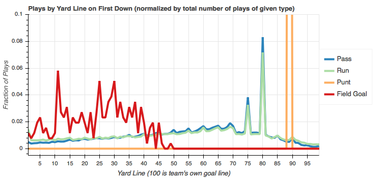
Aside from the single punt that happened on first down from the team's own 11 yard line, I don't see anything too surprising here. The slope of the pass line appears a little steeper than the run line. This indicates that the distribution of runs is skewed slightly more towards first down plays in good offensive position and the distribution of passes is skewed slightly more towards first down plays in poor field position in their own territory.
Second down
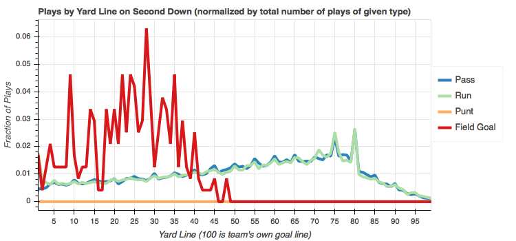
The distribution of passes and runs is shared pretty evenly along the entire field.
Third down
On third down, not surprisingly, passes are distributed more heavily towards plays in poor field position in a team's own territory. They're desperate for that first down. There were four punts on third down and two of them occurred within field goal range. I wonder what game situation forced that to happen. The data is all there in the CSV, but I'll leave that exercise up to the ambitious reader.
Fourth down
Like second down, there's a pretty similar distribution among passes and runs across the entire field which indicates that if the team doesn't punt or attempt a field goal, the pass/run ratio across the entire field is pretty much 1 to 1.
It's also interesting to see that the vast majority of fourth down runs start on the one yard line - almost 9% of all fourth down runs! I'd guess the increased number of plays, generally, at the one yard line is due to pass interference in the end zone. I'm curious what the touchdown conversion rate is for runs from the 1 yard line. Again, all the data's here, but I'm not going to dig on that one either.
Summary
In this post, I explored some NFL play-by-play data. You can find the data here. Since the data was already in such good condition, I didn't really have to do any cleaning. It was more of an exercise in Pandas slicing and filtering and plotting in Bokeh. In doing so, I tried to expose some interesting patterns in play type as a function of down and field location and I normalized the data both by the total numbers of plays at each yard line and also by the total number of plays of a given type across the entire field.
Hopefully you learned something! Please leave comments, questions, or found errors below. Thanks.
J253
Comments !